Daily electricity price forecasting (report)
Материал из MachineLearning.
(→Links) |
|||
| (9 промежуточных версий не показаны.) | |||
| Строка 79: | Строка 79: | ||
of non-hydro renewables capacity in the world, including the world’s largest | of non-hydro renewables capacity in the world, including the world’s largest | ||
operator of wind generation [7]. | operator of wind generation [7]. | ||
| - | |||
| - | |||
| - | |||
| - | |||
| - | |||
| - | |||
| - | |||
| - | |||
| - | |||
| - | |||
| - | |||
| - | |||
| - | |||
| - | |||
| - | |||
| - | |||
| - | |||
| - | |||
| - | |||
=== Basic hypotheses and estimations === | === Basic hypotheses and estimations === | ||
| Строка 711: | Строка 692: | ||
! width=30 % |# | ! width=30 % |# | ||
! width=160 % | Description | ! width=160 % | Description | ||
| - | |||
| - | |||
|- | |- | ||
| '''1''' || time series | | '''1''' || time series | ||
| Строка 736: | Строка 715: | ||
| '''26''' || wind speed | | '''26''' || wind speed | ||
|- | |- | ||
| - | |} | + | |} |
| - | + | ||
| - | + | ||
| - | + | ||
====Experiments with simple LARS==== | ====Experiments with simple LARS==== | ||
| Строка 1005: | Строка 981: | ||
! width=50 % | DOW LARS | ! width=50 % | DOW LARS | ||
! width=50 % | LAF | ! width=50 % | LAF | ||
| - | |||
| - | |||
|- | |- | ||
| '''MAPE''' || 16.64% || 15.29% || 13.31% || 14.79% || 20.43% | | '''MAPE''' || 16.64% || 15.29% || 13.31% || 14.79% || 20.43% | ||
| Строка 1050: | Строка 1024: | ||
LARS. We also created realization of local algorithm | LARS. We also created realization of local algorithm | ||
k-nearest-neighbours to compare results. | k-nearest-neighbours to compare results. | ||
| + | |||
| + | == Look also == | ||
| + | |||
| + | [[Прогнозирование ежедневных цен на электроэнергию (отчет)]] is brief explanation of this report in russian. | ||
| + | |||
| + | [[LARS]] | ||
| + | |||
| + | [[Метод k ближайших соседей (пример)]] | ||
| + | |||
| + | ==Links== | ||
| + | |||
| + | [https://mlalgorithms.svn.sourceforge.net/svnroot/mlalgorithms/Group674/Zaitsev2009DEPF/ Project report, architecture and system files] | ||
== Bibliography == | == Bibliography == | ||
| Строка 1123: | Строка 1109: | ||
}} | }} | ||
| - | {{ | + | {{ЗаданиеВыполнено|Зайцев Алексей|В.В. Стрижов|15 декабря 2009|Likz|Strijov|}} |
__NOTOC__ | __NOTOC__ | ||
| + | [[Категория:Практика и вычислительные эксперименты]] | ||
Текущая версия
Project description
Goal
The goal is to forecast average daily spot price of electricity. Forecasting horizon (the maximal time segment where the forecast error does not exceed given value) is supposed to be one month.
Motivation
For example, one needs precise forecast of electricity consumption for each hour during the next day to avoid transactions on the balancing market.
Data
Daily time series from 1/1/2003 until now. Time series are weather (average-, low-, and high daily temperature, relative humidity, precipitation, wind speed, heating-, and cooling degree day) and average daily price of electricity. There is no data on electricity consumption and energy units prices. The data on sunrise and sunset are coming from the internet.
Quality
The time series splits into the whole history but the last month and the last month. The model is created using the first part and tested with the second. The procedure must be repeated for each month of the last year. The target function is MAPE (mean absolute percentage error) for given month.
Requirements
The monthly error of obtained model must not exceed the error of the existing model, same to customers. It’s LASSO with some modifications.
Feasibility
The average daily price of electricity contains peaks and it is seems there is no information about these peaks in given data. There is no visible correlation between data and responses.
Methods
The model to be generated is a linear combination of selected features. Each primitive feature (of index j) is a set of j+nk-th samples of time series, k is a period. The set of the features includes primitive features and their superpositions.
Problem definition
We have variables matrix and responses vector
for this matrix. This is
time series. Our goal is to recover regression
for variables matrix
. This
data is straight after initial data in time. Our goal is to find vector
of linear
coefficients between
and
,
.
As quality functional we use MAPE (mean average percent error).
,
Algorithm description
State of art
The main task of this subsection is to describe ways of daily electricity price
forecasting and sort of data needed for this task. Also we have a deal with
German electricity price market and there is brief survey about it.
Let’s start from methods of forecasting daily electricity price. There are
many ways to solve this problem. It can be ARIMA models or autoregression
[1], [4]. Artificial neural networks are also used in combination with some serious
improvements like wavelet techniques or ARIMA models [2]. SVM can be used
in a close problem of price spikes forecasting [2]. Models of noise and jump can
be constructed in some other ways [3].
Sets of data can be rather different. For neural networks it can be only
time series [1], but in most of works some addition data is required. Weather is
an important factor in price forecasting [5]. It can be median day temperature,
HDD, CDD [4] or wind speed [6]. Dates of sunsets and sunrises can be useful too.
Energy consumption and system load has important impact on daily electricity
price [4]. Interesting features is prediction instead of
electricity
price in €.
Our goal is forecasting daily electricity price for German electricity price
market EEX, so let’s represent some information about it. Germany has free
2
electricity market, so models for free electricity market can be applied to it.
Market of energy producing changes every year, main goals are phasing out
nuclear energy and creation new renewable sources manufactures. Germany is
one of the largest consumers of energy in the world. In 2008, it consumed energy
from the following sources: oil (34.8%), coal including lignite (24.2%), natural
gas (22.1%), nuclear (11.6%), renewables (1.6%), and other (5.8%), whereas
renewable energy is far more present in produced energy, since Germany imports
about two thirds of its energy. This country is the world’s largest operators
of non-hydro renewables capacity in the world, including the world’s largest
operator of wind generation [7].
Basic hypotheses and estimations
In case of linear regression we assume, that vector of responses is linear
combination for modified incoming matrix of features
, what we designate as
:
.
This modified matrix we can get from superposition, smoothing and autoregression in initial data set. LARS[8] seems suitable for this kind of problem, so we use it in our work. From state of art and data we get some additional hypotheses. We have a deal with data set with two periodic – week periodic and year periodic. Possible usage of this is generation new features and creation own model for each day of week.
Mathematic algorithm description
LARS overview
LARS (Least angle regression \cite{[9]}) is new (2002) model selection algorithm. It has several advantages:
- It does less steps then older LASSO and Forward selection.
- This algorithm gives same results as LASSO and Forward selection after simple modification.
- It creates a connection between LASSO and Forward selection.
Let's describe LARS. We have initial data set , where
is number of variables,
is number of objects.
is responses
vector. Our goal is recovery regression and make estimation for
, where
For each algorithm step we add new variable to model and create parameters estimation for variables
subset. Finally we'll get set of parameters estimation
. Algorithm works in condition of independence
.
Describe this algorithm single step. For subset of vectors with the largest correlations, we add one vector to it,
and get indexes set . Then
where . Introduce
where --- ones vector size
. Then calculate equiangular vector between
:
Vector has equal angles with all vectors from
After introducing all necessary designation one describe LARS. As
Stagewise, our algorithm starts from responses vector estimation
. After that it makes consecutive
steps in equiangular vector dimension. For each step we have
with estimation :
Get active vectors indexes set from
Introduce additional vector:
Write next approximation for estimation
where
This actions do
minimization step for all variables with
indexes from set <\tex>A</tex>. In addition
is the least
positive
on condition that we add new index to
on
the next step :
This algorithm works only steps. The experiment in article
\cite{[1]} confirms, that LARS works better LASSO and Forward
Selection, and makes less number of iterations. Last step
estimation gives least-squares solution.
Apply LARS
We use three steps in this algorithm.
- Modify of initial data set
and set to classify
. Get
.
- LARS algorithm apply.
- We split our initial sample into two parts: for learning and for control
.
- For learning sample we apply procedure of removing spikes from this part of sample.
- From we get a set of weights vectors
for each step of LARS
algorithm.
- By using control sample we choose
with best MAPE rate.
- Calculate
.
Local algorithm Fedorovoy description
This algorithm is variation of k-means for time series. We have
time series . Suppose continuation of
time series depends on preceding events
. Select in our set subsets
Introduce way to calculate distance
between
and
.
Define set of linear transformations for
:
Note that for our problem importance of objects increases to the
end of vector because of forecasting straightforward
vector
. Introduce parameter
. So,
our distance
is
where
From that distance definition find closest elements to
. We use this set of elements
, sorted by ascending of
, to create forecast by equation
for each , where
proportional to distances
So ,we use integrated local averaged method to create forecast.
This algorithm needs optimization by several parameters and it's
not useful without this procedure \cite{[11]}. Our model requires
(
is fixed and equals one month length ). To
define them we use two step iteration process from
:
- Optimization by
.
- Optimization by
.
It's necessary to keep in mind, that we use specified model of
general algorithm from \cite{[11]}. Function of distance and
weights for each element from set of can be chosen
from another basic assumptions.
Apply Local algorithm Fedorovoy
For Local algorithm Fedorovoy we use only responses vector . To
forecast future responses we have to initialize and optimize
parameters of this algorithm (see section above).
- Optimize parameters
,
for algorithm
- Apply algorithm for last
elements of our responses set
Set of algorithm variants and modifications
LARS algorithm works steps, where
is number of variables
in matrix
. Expanding number of variables linear increases time
for the algorithm to work. Let's introduce construction of new
variables generation.
- initial set of variables.
\smallskip
- set of primitive functions so
called primitives with argument from
and subset of
.
\smallskip
- new set of variables. For
each variable
where is superposition of functions from
.
For our algorithm initial set of variables is . We introduce
set of primitive functions from several components.
Numericals operations
First component consists of simple numerical operations. For
example, square rooting or cubing. We add arithmetical operations
like addition and multiplication. Superposition of this functions
can be used in our new variables matrix .
Smoothing function
Second component consists of smoothing functions. We use Parzen
window smoothing with two parameters: width of Parzen window
and periodic
. For each element from sample we calculate
for each object, where
,
is indexes of elements from data
set. Only condition for
is
. In our case we use one from set of different kernel
functions. It is Epanechnikov kernel function.
, where
is normalization
coefficient,
. There is periodic with
step 7 in data set. For responses data set it seems reasonable
apply kernel smoothing several times for windows with different
periodic
.
Autoregression
In our model we add autoregression to set of primitive functions
from variables and responses. For each variable adding we use
parameters -- shift of data.
for each object, where are indexes from data matrix. For
objects in sample to classify we have to calculate it step by step
for responses. If there is no value for
,
, we
have to assign this value to be zero. It decreases correlation
value for this autoregression variable in LARS algorithm. But our
sample has about three thousands elements and for small values of
,
, this factor decreases correlation in rate about
or smaller in average.
As alternative we use another way to create autoregression matrix.
There are periodicals in our data set. To reshape our answers
matrix we create the set of new variables from responses. For
periodical length choose
. Then create
model for each part of periodical. From full sample of row indexes
select
. In set of
matrixes for each
we get from LARS its own
model of linear regression. Otherwise, we modify our variables
matrix according to scheme
First row is indexes, what we leave in our variables matrix. To the right of them is variables, which we add to new variables matrix.
Removing spikes
Another primitive function in our set is procedure of removing
spikes from our sample. This function uses two parameters. It's
maximum rate of first and second type errors . At first
step our algorithm classify all sample by using this initial
sample
. At second step we removing objects from sample if rate
of error to true value
or if rate of error to responses mean value
We get from crossvalidation: 12 times we split sample
to control and learning sample. For learning sample we create
forecast to control sample. By optimization
we get minimum of
mean MAPE for control set.
Normalization
For some variables we need normalization. This primitive function is necessary in our sample. It can be
for each from
. This normalization makes nearly
equal initial conditions for each variable in LARS and that is we
need. This primitive is useful for responses and variables.
Additional notes
It's necessary to make some additional notes. Some functions can be useful only for subset of variables and we have to take into account this fact. Another thing to pay attention is a possible usage primitives superposition.
All this statements need additional researching and computing experiments in other parts of this article to create good model for our problem.
System description
In this section our goal is to give system description, its components and organization. Mathematical algorithm descriptions and applying this system to our problem lie out of this section.
System overview
Project architecture description
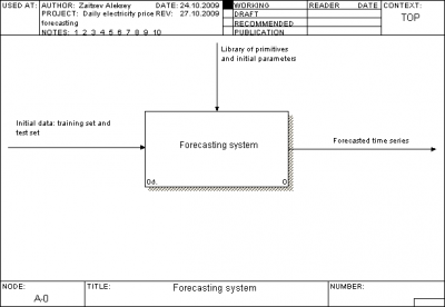
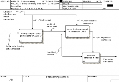
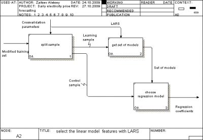
We use standard IDEF0 for our project architecture description. One can view it in format .bp1 outside this report or look to figures below.
For our problem we have test set and training set. Our task is get
responses for test set by using training set with known responses.
We have three main activity box tools to create forecast. They are
depicted at second figure. First creates modified data set
from initial data set. For test set it generates set of additional
variables. For training set it modifies variables and remove
outliers (spikes) from our set. Work of second is depicted on
third figure. At first we split our training set to learning and
control sets. After that second activity block tool
create a
set of models by using learning set and chooses best by using
control set. So, we have a regression model from
. We apply it
in
to our test set to get responses for this set.
System organization description
For our system we split our system files into two main folders and two files in root of our problem folder.
- ModelElectricity.bp1 -- system description in .bp1 format for IDEF0 standard.
- Project report.pdf -- document you are reading now
- Algorithms -- set of algorithms we have apply to our problem (DOW LARS, Local algorithm Fedorovoy, LARS)
- Plots contains results for each algorithm and model we applied, tests for algorithm modules and system architecture in .bmp.
Data representation
Fotr all algorithms we use data from file DayElectricityPrice.mat, what contains
| Name | Size | Description |
|---|---|---|
| xRegression | | variables matrix |
| yRegression | | responses matrix |
For each element from we assume, that it is integer or real value, and first column for each matrix is time series.
To run algorithm DOW LARS and LARS we have to modify data to form with synchronized time series:
| Name | Size | Description |
|---|---|---|
| trainingX | | training variables matrix |
| trainingY | | training responses vector |
| testX | | test variables matrix |
| model | | algorithm parameters vector |
For Local algorithm Fedorovoy we don't use model vector and
variables matrix.
| Name | Size | Description |
|---|---|---|
| trainingY | | training responses vector |
| testX | int | forecasting horizon |
| | | algorithm parameters |
If data meets requirements in this tables, one can run units to calculate responses for test set.
Units description
| Algorithm | MATLab file | Description |
|---|---|---|
| LARS | LARS.m,modLARS.m | realize LARS |
| Local algorithm Fedorovoy | kMeans.m | realize LAF |
Each unit is commented and describe its'way of work. To run them
one has to go to certain folder and run Demo.m to understand
algorithm work by a number of examples.
Tests description
For each units we created a number of tests. Each test has to check certain property of algorithm and get to us information about its'work for model set of data.
LARS
Let's check algorithms for set of simple model cases. In each case we use same crossvalidation procedure and sample of objects. We have 100 objects and 20 variables. Our goal is to forecast 10 times 5 forward objects. Control sample we create by removing last objects from initial sample. For each new step learning sample is shorter, then old by 5 objects. Results are collected in the table after all cases description.
First case is linear dependence responses from variables.
X = rand(100,20)-0.5;
beta = rand(1,20)-0.5;
Y = X*betaInit';
In second case dependence is quartic.
X = rand(100,20);
beta = rand(1,20);
Y = (X.*X)*betaInit';
In third case we add normal noise to variables.
X = rand(100,20);
beta = rand(1,20);
Y = X*betaInit';
X = X + (rand(100,20)-0.5)/2;
For each case we calculated mean MAPE(1) for set of crossvalidation procedures. Results are in the below table. They are confirmation of our LARS realization correctness. For each case we got expected results. First case was simple for the algorithm. It recreate linear dependence responses from variables. In second case principal inadequacy of our model for given problem gave MAPE equals 0.073 in forecasting. For third case principal impossibility to predict noise led to error rate MAPE 0.065.
| Case number | 1 | 2 | 3 |
|---|---|---|---|
| MAPE | near 0 | 0.073 | 0.065 |
Local algorithm Fedorovoy
This algorithm has to be good for near to periodic data, where responses in future depend on past responses. We use model data to test our algorithm. First test has to be simple for this algorithm:
m = 1:400;
initY = sin(m)'; % responses
n = 6; % number of crossvalidation procedures
t = 30; % forecasting forward horizon
k = 7; % k for k nearest neighbours method
w = 0.9; % weight in calculating distance
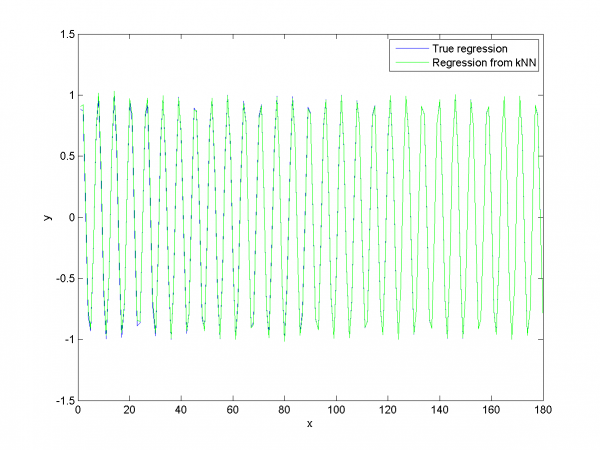
For second test generated data included two periodics with increasing amplitude.
m = 1:400;
initY = (m.*sin(m).*sin(0.1*m))';  % responses
n = 6; % number of crossvalidation procedures
t = 30; % forecasting forward horizon
k = 7; % k for k nearest neighbours method
w = 0.9; % weight in calculating distance
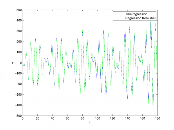
Results for this test are depicted on the plot below:
We apply our algorithm for two model data sets. It works good if data obeys hypothesis about dependence of future data set from past data set.
Computing experiment report
Visual analysis
Model data
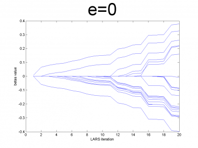
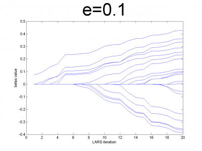
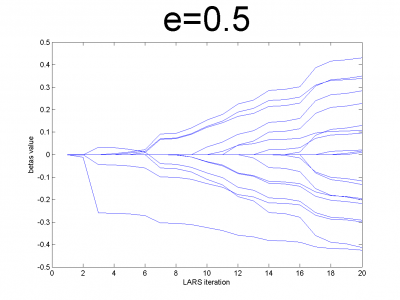
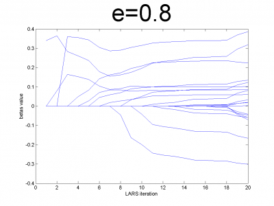
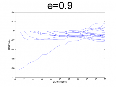
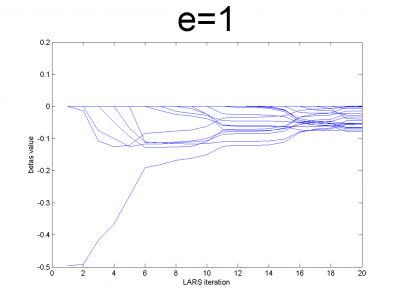
At first we have to test our interpretation of LARS to be sure
about its correct work. LARS has to work better with
well-conditioned matrix, as many linear algorithms, such as LASSO.
For ill-conditioned matrix values of regression coefficients
appear to increase and decrease during each step of
algorithm. We generate model data by the below code.
n = 100;
m = 20;
X = e*ones(n,m)+(1-e)*[diag(ones(m,1));zeros(n-m,m)];
beta = (rand(m,1)-0.5);
Y = X*beta;
X = X + (rand(n,m) - 0.5)/10;
For different values of we get ill- and well-conditioned
matrices. We use
. If
is small
matrix'll be well-conditioned with close to orthogonal correlation
vectors, if
is close to 1, we get matrix from just ones with
little noise. This matrix is ill-conditioned. Directions of
correlation vectors are near to same.
So, our LARS realization works normal according to this property.
Data description
As real data we use set from our problem. It consists
from variables matrix and responses vector
. We will designate them as
and
. Size of
is
, where
is number of objects (time series from
days) and
is number of variables for each object. Size of
is column
.
First column for both and
is time series. For
second
column is responses for each object from
. They are normalized
by year mean. Number of variables in
is 26. They are described
in below table.
| # | Description |
|---|---|
| 1 | time series |
| 2-6 | day of week |
| 7-18 | month |
| 19 | mean temperature |
| 20 | HDD |
| 21 | CDD |
| 22 | high tepmeratue |
| 23 | low temperature |
| 24 | relative humidity |
| 25 | precipitation |
| 26 | wind speed |
Experiments with simple LARS
We do a number of computational experiments with real data. For each experiment we calculate MAPE value.
In first case we use simple LARS algorithm without any additional
improvements for matrix and column
.
model = [1,1,0,0,0,0,0,0,0]; % model parameters
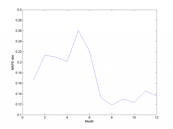
Mean MAPE for all months equals 16.64%.
For second experiment we use some additional variables. They are squares and square roots from basic variables
model = [1,1,1,0,0,0,0,0,0]; % model parameters
Mean MAPE for all months equals 17.20%.
In third experiment we use smoothed and indicator variables.
model = [1,0,0,1,0,0,0,0,0]; % model parameters
Mean MAPE equals 17.16%.
For the next experiment we choose smoothed and squared smoothed variables.
model = [1,0,0,1,1,0,0,0,0]; % model parameters
MAPE equals 19.2%.
In the last experiment of this subsection we choose combination of nonsmoothed and smoothed variables.
model = [1,1,1,1,0,0,0,0,0]; % model parameters
We get MAPE 16.89% in this experiment.
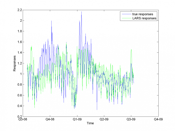
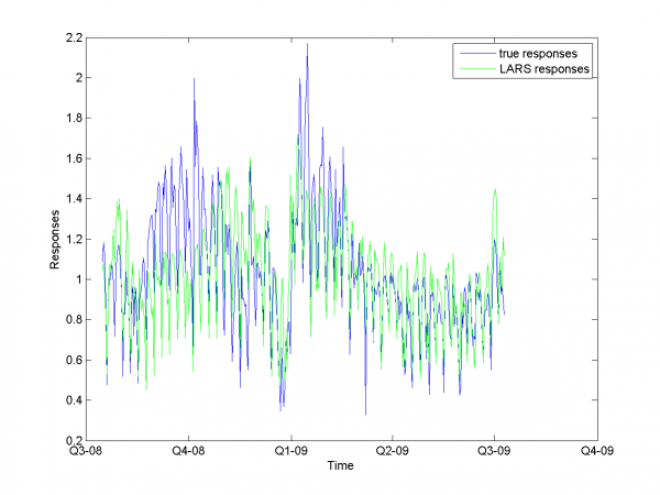
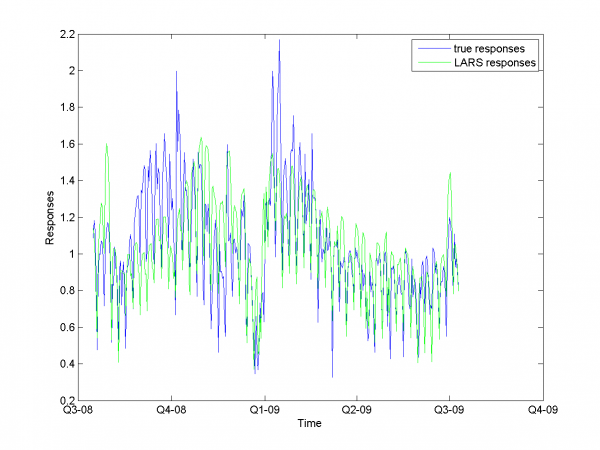
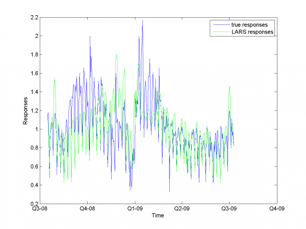
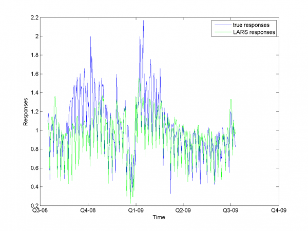
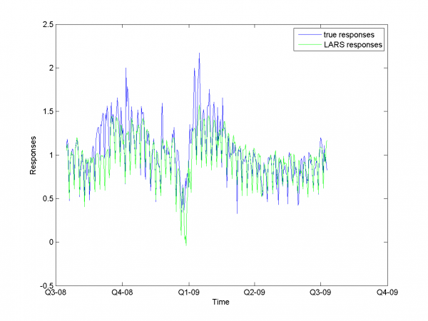
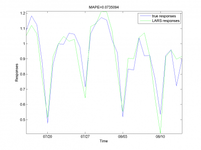
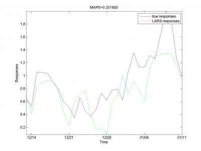
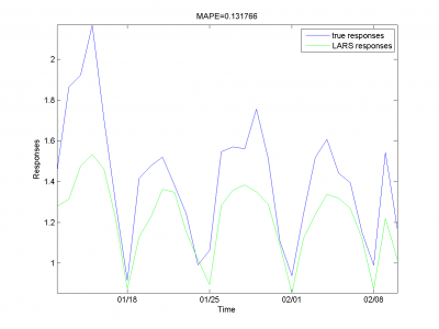
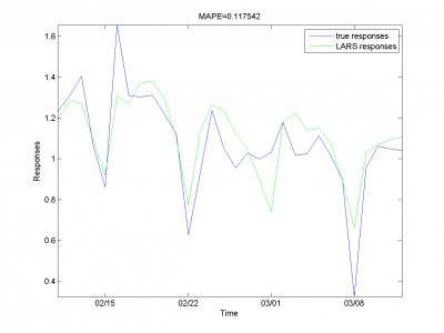
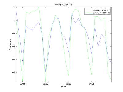
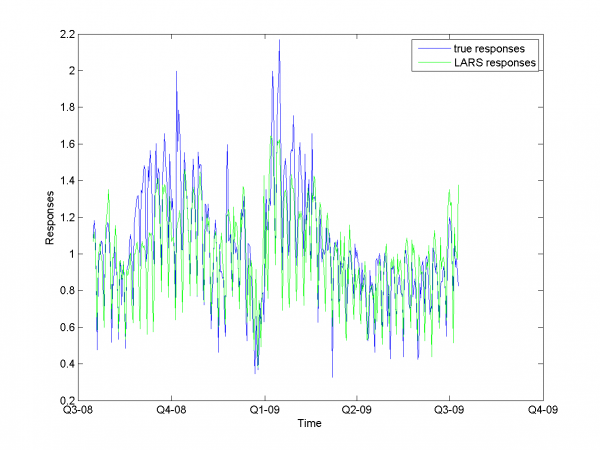
From experiments above we draw a conclusion, that for simple linear method LARS MAPE is in bounds of 16-18%. Adding smoothed variables can't correct situation. From plots one can see problem of spikes prediction. MAPE for unexpected jumps is bigger, then MAPE for stationary zones. To increase accuracy of our forecast we need another methods.
Removing spikes
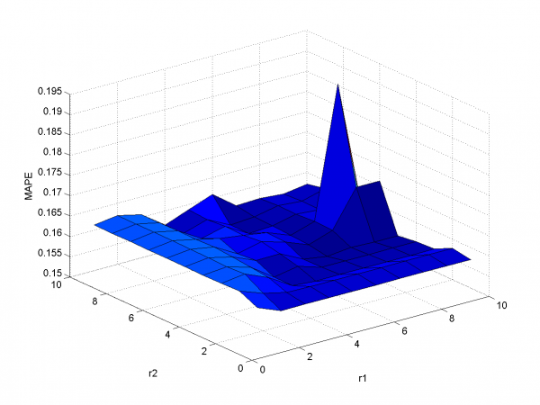
To create better forecast we need to remove outliers from learning sample. This procedure helps to get better regression coefficients. In our case remove spikes procedure depends on our basic algorithm model and two parameters. To get optimal value of this parameters we use 2 dimensional minimization MAPE procedure.
First experiment uses initial variables and removing spikes procedure.
model = [1,1,0,0,0,0,0,0,0]; % model parameters
Minimum MAPE equals 15.45\%. It is in point
. MAPE is smaller, then gained in
previous subsection.
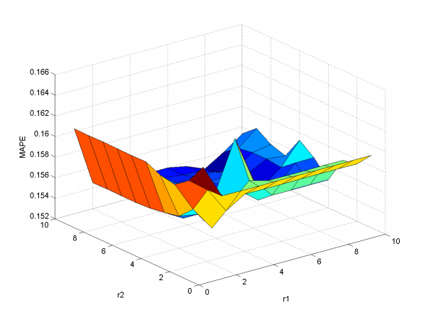
In second experiment we use another model. We add modified initial variables and smoothed variables.
model = [1,1,1,1,0,0,0,0,0]; % model parameters
MAPE function has local minimum in point
and equals 15.29%. Let's look to plots for optimal
and
.
Removing outliers doesn't help us to get better result for months with unexpected behavior. To the end of this subsection we note, that this procedure gives us advantage in competition with previously obtained models and algorithms in previous subsection. Best MAPE rate for this section experiments is 15.29%.
Autoregression
Add autoregression according to subsection {\bf 3.4.3} is sound idea for many forecasting algorithms. We use autoregression in two ways.
First way is add to each day from sample responses for days in past and forecast responses for extended variables matrix. As in previous subsection we use 2-dimensional discrete optimization for removing spikes parameters.
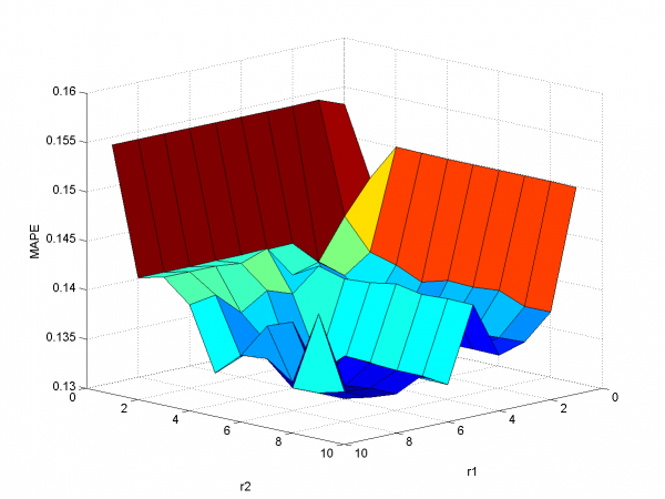
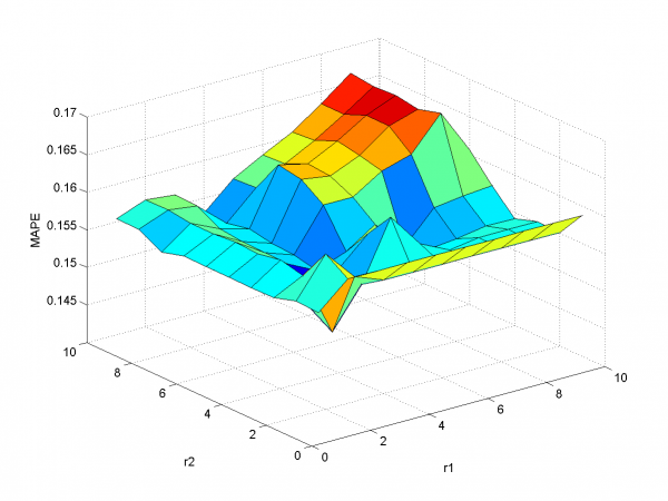
We change standard point of view to get more convenient to view
surface. Minimum MAPE value is in point .
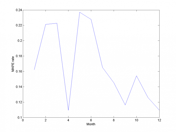
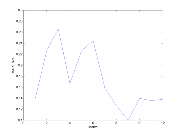
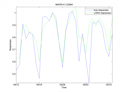
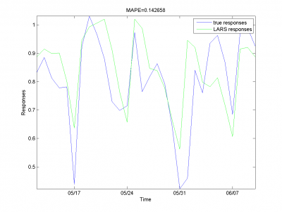
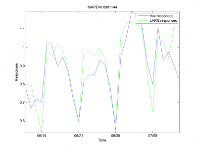
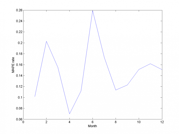
It equals 13.31%.
model = [1,1,1,1,0,0,0,0.7,0.8]; % model parameters
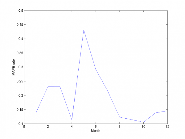
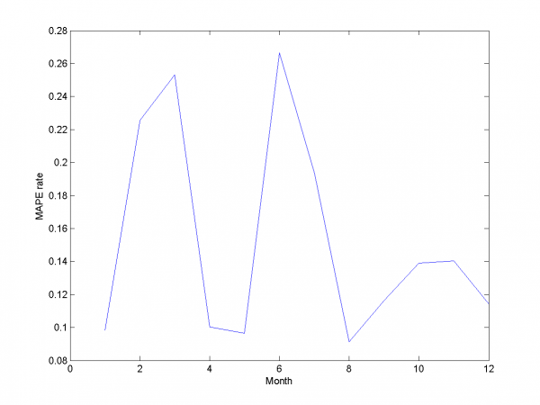
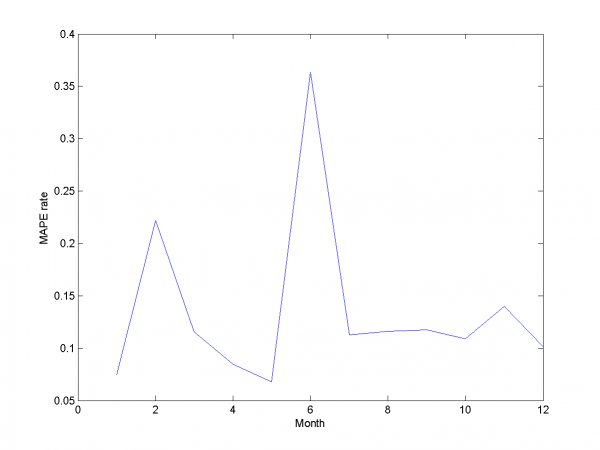
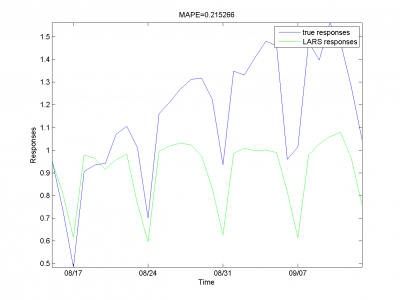
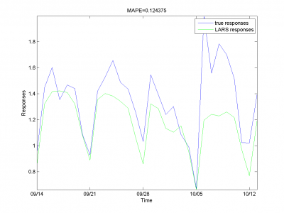
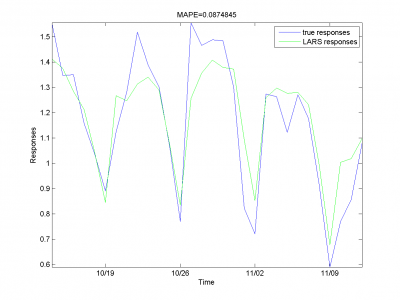
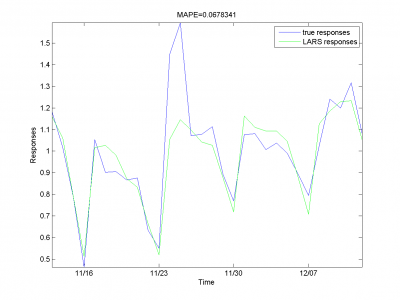
And for each month:
For this experiment we have best results from our set of different models algorithm. But to complete article it's necessary to analyze work for other algorithm and models we have use during work.
Set of models for each day of week
In data set with periodics can be suitable create it's own model for each element from periodic. For example, we can create different regression models for different dais of week. Work of this heuristic in our case seems interesting.
In experiments we split in two parts: for control and for test. We forecast 4 day of week forward for each day. So, we create for each crossvalidation forecast for 28 days.
In first case we create model from standard variables. We test our
sample with different size of test sample (by what we choose best
). Motivation of this step is small number of elements in
control sample. It equals 4. But for different sizes of test set
there is no decreasing of MAPE effect.
model = [1,1,1,1,0,0,0,0,0,s]; % model parameters
is multitude to create size of test sample. Size of test set
equals
.
| Control set size | 4 | 8 | 12 | 16 | 20 | 24 | 28 | 32 | 36 | 40 |
|---|---|---|---|---|---|---|---|---|---|---|
| MAPE rate | 0.1740 | 0.1860 | 0.1790 | 0.1897 | 0.184 | 0.1826 | 0.1882 | 0.1831 | 0.1846 | 0.195 |
From this table one can see, that results for this experiment
aren't better, then results for model without choosing individual
model for each day of week.
Let's add autoregression matrix to this model according to way we
describe in 3.4.3. We get from
two-dimensional optimization by this parameters.
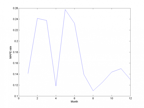
We got results below. MAPE equals 14.79\%.
model = [1,1,1,0,0,0,6,0.3,0.3,1]; % model parameters
To the end of this section we say, that for our data set this way can't give us as precise results as method from previous section.
Local algorithm Fedorovoy
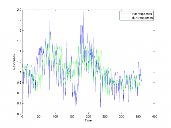
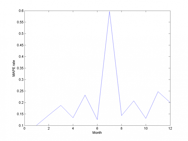
For algorithm Fedorovoy we don't use any additional hypotheses except described in works \cite{[11]},\cite{[12]}. Results for this algorithm are worse, that result for different LARS variations. Main complications in our data for this algorithm are big noises and spikes in learning and test data set and weak dependence future data from past. Motivation to use this algorithm is periodics in our data.
To get parameters for this algorithm we have used iteration
method. At first iteration we got local minimum in point , where
is number of nearest neighbours for our
algorithm and
defines way to calculate distance between
different segments of our sample.
MAPE equals 20.43%.
Criterion analysis
We use MAPE quality functional. In our case target function to minimize is deviation of initial responses to ones from algorithm, so this functional looks suitable. For many variations and 2 algorithms we got set of different results. Let's briefly describe them in the table.
| Algorithm | LARS | RS LARS | RS and autoLARS | DOW LARS | LAF |
|---|---|---|---|---|---|
| MAPE | 16.64% | 15.29% | 13.31% | 14.79% | 20.43% |
LARS is simple LARS realization with best set of variables. AutoLARS is LARS with removing spikes procedure. RS and autoLARS is LARS with removing spikes and adding autoregression variables. DOW LARS is LARS with creation specified model for each periodic (in our case -- week periodic). For this algorithm we also add autoregression variables and remove spikes procedure.LAF is local algorithm Fedorovoy realization. For our variants of this algorithms set we get best result with RS and autoLARS.
Main complication for most of algorithm was spikes and outliers in data set. Another complication for LARS-based algorithm was weak correlation between initial variables and responses. To this problem we add also high rate of noise. The reason of it can be unobservable in our data events. Some from our algoithms take into account this complications. They gave us better results, then simple algorithms. But we get only 4-5% of MAPE rate by applying our best algorithm in complication with simple LARS.
Dependency from parameters analysis
In different sections of our work we use a number of optimization procedures. Frow plots and 3d plots one can see, that all optimizations are stabile and give us close to optimal parameters. In most algorithms we use simple discrete one- or two-dimensional optimization. For local algorithm Fedorovoy we use iterations method, but he gives us local optimum result at first step. May be, it's suitable to apply randomization search in this case.
Results report
For our best algorithm we decrease MAPE rate by 5% from initial algorithm (We get 13.31% MAPE rate vs 17% in start). To solve this problem we applied big set of heuristics and modifications to LARS. We also created realization of local algorithm k-nearest-neighbours to compare results.
Look also
Прогнозирование ежедневных цен на электроэнергию (отчет) is brief explanation of this report in russian.
Метод k ближайших соседей (пример)
Links
Project report, architecture and system files
Bibliography
- Hsiao-Tien Pao A Neural Network Approach to m-Daily-Ahead Electricity Price Prediction. — 2006.
- Wei Wu, Jianzhong Zhou,Li Mo and Chengjun Zhu Forecasting Electricity Market Price Spikes Based on Bayesian Expert with Support Vector Machines. — 2006.
- S.Borovkova, J.Permana Modelling electricity prices by the potential jump-diffusion. — 2006.
- R.Weron, A.Misiorek Forecasting spot electricity prices: A comparison of parametric and semiparametric time series models. — 2008.
- J.Cherry, H.Cullen, M.Vissbeck, A.Small and C.Uvo Impacts of the North Atlantic Oscillation on Scandinavian Hydropower Production and Energy Markets. — 2005.
- Yuji Yamada Optimal Hedging of Prediction Errors Using Prediction Errors. — 2008.
- Wikipedia.
- Bradley Efron, Trevor Hastie, Iain Johnstone and Robert Tibshirani Least Angle Regression. — 2002.
- Robert Tibshirani Regression shrinkage selection and via the LASSO. — 1996.
- Vadim Strijov Model Generation and its Applications in Financial Sector. — 2009.
- J. McNames Innovations in local modeling for time series prediction. — 1996.
- В. Федорова Локальные методы прогнозирования временных рядов. — 2009.
| | Данная статья была создана в рамках учебного задания.
См. также методические указания по использованию Ресурса MachineLearning.ru в учебном процессе. |
