Повышение точности прогнозов на данных Netflix с помощью построения алгоритмических композиций (отчет)
Материал из MachineLearning.
(→System description and report) |
|||
| Строка 235: | Строка 235: | ||
== System description and report == | == System description and report == | ||
| - | * Link to [https://mlalgorithms.svn.sourceforge.net/svnroot/mlalgorithms/Spirin2009Netflix/ the same file in a pdf format] | + | * Link to [https://mlalgorithms.svn.sourceforge.net/svnroot/mlalgorithms/Group674/Spirin2009Netflix/ the same file in a pdf format] |
== See also == | == See also == | ||
Текущая версия
Project Specifications
The Goal
Boost the performance of existing algorithms on Netflix data with the help of algebraic approach to the synthesis of algorithmic compositions.
The Motivation
There is a possibility exists that individually weak algorithms while used in a compositions could result in a much better performance. There has been left a lot of probes (according to Netflix's notation) after the Netflix Prize. So, it would be interesting to apply algebraic approach to combine them and achieve better accuracy.
The Data
The data comes from 1,151 sets of predictions of integer ratings in the range (1-5). Each set of predictions was generated by algorithms with the objective to minimize the RMSE over the full set of over 1.4 million ratings. All the individual probe files were merged into one large file (1,151 columns, 1.4 million rows). From this file, random sampling was used to generate data sets. Each of the data sets is split into 2 files, one for Training (Rating provided) and one for Scoring. There are 2 small and 2 medium data sets.
In each of the data sets, the Training and Scoring files are of the same size:
- RMSE — 200 sets of predictions for 15,000 ratings. The objective is to minimize the RMSE.
- AUC — 200 sets of prediction for 15,000 ratings. Only ratings of 2 particular values are included (e.g. 1s and 5s), sampled with different weightings on each value. The objective is to minimize the AUC.
The data sets are csv files with header rows. The first 2 columns are rowID and Target (actual rating) and then 200 columns of predicted rating values. In the Scoring files the Target values are zeros. For both the RMSE and AUC datasets, the predicted ratings values have been converted to integers by rounding to 3 decimal places and multiplying by 1,000. Thus each predicted rating will be an integer and should lie in the range 1,000 to 5,000. The author thanks AusDM committee for datasets and ability to check predictions after the competition final.
Evaluation Criteria
- RMSE (http://en.wikipedia.org/wiki/Mean_squared_error)
- AUC (http://en.wikipedia.org/wiki/Receiver_operating_characteristic)
For the AUC dataset, the Target values are 1 and -1 (zeros in the Scoring files).
Therefore, in this case Netflix Dataset was modified so that to allow 2-class recognition (where 1~5stars and -1~1star)
Requirements
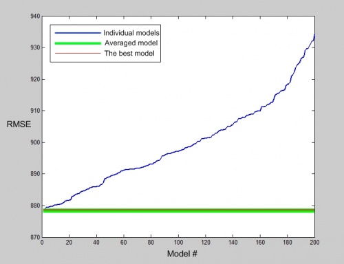
Synthesized algorithms should at least outperform simple averaged composition.
Feasibility and Possible Obstacles
We can only assess the diversity of algorithms but we don't know the underlying principle of how any given algorithm has been trained and what kinds of correlations exist among algorithms. “A necessary and sufficient condition for an ensemble of classifiers to be more accurate than any of its individual members is if the classifiers are accurate and diverse”. Dietterich (2000)
Approach
Genetic Algorithm, Stochastical Local Search with Adaptation, (For|Back)ward Stepwise Selection (Greedy Search), Logistic Regression, Bagging
Mathematical Formalization of the Problem
Given a set of predictions (e.g. Netflix' probes) for finite set of samples - an matrix, and the true labels -
vector. Build a correcting operator in the space of all functions over initial space F that will give better performance on a qualifying (test) set. Initial dataset was partitioned into two independent datasets: training and qualifying.
Hypotheses about underlying data properties
All probe-predictions yield performance better than simple random guessing algorithm (in case of classification problem), and uniform predictions over the set of (1:5) in Z (in case of regression problem). Distribution of labels in training and qualifying sets is the same. Because of all probes has been built by well-known scientists and they have used stable and robust algorithmic models, all probes are informative. We can treat this problem as a problem of feature selection where each probe-prediction is a unique feature. Therefore, backward stepwise selection should yield better results. On the contrary forward stepwise selection is unstable when there are a lot of “good” models [6,7].
Descriptions of the Algorithms
Forward Stepwise Selection (FSS)
Take the best algorithm (based on a CV procedure). Then sequentially add algorithms to the composition that maximize a performance measure at each step. At each iteration memorize the value of performance measure so that to identify the best set of algorithms. Stop the process when there are no algorithms that can boost the performance of a current composition. Return a set of algorithms’ indices that lead to the best performance on an independent test set. Report
Heuristics and Modifications
From the experiments one can notice that this process is unstable and stops just after a few iterations. This is because of the greedy nature of the FSS-algorithm. To soften the greedy search one can continue the composition building process d more iterations and then find the best one. In this case we give the chance to the FSS-algorithm to postpone termination. A few heuristics come from Caruana et al. [?]. Firstly, they suggest initializing the process with N best models and then adding algorithms as it is described above. Secondly, they recommend allowing algorithms to be added to the composition more than once. “Selection with replacement allows selection to continue adding copies of good models instead of being forced to add inferior models”. In addition, all these techniques combat overfitting.
Backward Stepwise Selection (BSS)
The algorithm works almost in the same manner but now instead of adding algorithms to the composition it excludes them. The composition is initialized with the full set of individual algorithms. Report
Forward-Backward Stepwise Selection (FBSS)
The idea is to combine two greedy strategies together and hence to find better solution. The FBSS –algorithm is initialized as the FSS. Then it works as FSS during the forward stage. But instead of breaking the process of composition building, it runs d more iterations, and then starts working in reverse direction (starts excluding less-useful for composition algorithms). The annihilation process continues d iterations and then the FBSS algorithm switches to the forward stage. This happens s times and then the algorithm returns the optimal set of base models among all sets that has been considered. Report
Breadth-First Search Pruned (MultiRow Iterative Search, Group Method of Data Handling, GMDH)
The FSS-algorithm adds the model that leads to better performance in a current iteration. Of course, it is a reasonable step, but at the same time it is reasonable only locally. Because the situation might happen during the next iteration that the composition built by greedy strategy is worse than another composition of the same size. And the underlying restriction is that the FSS-algorithm builds only one composition. Here we suggest to build B compositions and finally to find the best one after d iterations. The pseudocode is shown below. Report
Genetic Algorithm (GA)
According to Darwin’s Principle only successful individuals go to the next generation. Each composition is coded by indicator vector that tells us which base algorithms are used. The measure of success is a CV based value that helps to find compositions capable of predicting targets for a new data with low error rate. Additional information is available in GeneticSearchReport.m. Report
Internal Model
Depending on a problem two different internal models are used. For the AUC task we have implemented the logistic regression training method and consider 3 ways of composition building (FSS, GMDH, GA). In case of the RMSE task we use simple averaging as a blending method and have implemented 5 algorithms for composition construction (FSS, BSS, FBSS, GMDH, GA). Because of time restrictions and available computing power we have decided not to build compositions with BSS and FBSS for the AUC (the BSS algorithm starts with the full set of features/predictions and that is why it needs a lot of time to build logit model and find the best value and corresponding set of indices even at first stages).
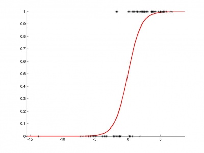
Logistic Regression
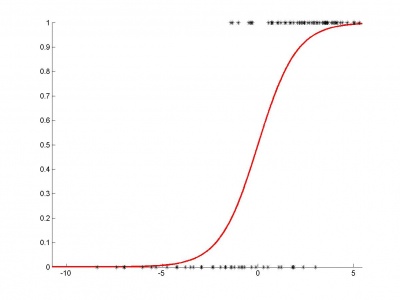
To construct a two-class response we use logistic regression where each probe file is treated as a feature. Here we use a Newton-Rawson method to find the local minimum of the functional (AUC).
Mathematical Foundations
Basically, all these algorithms tend to optimize the full search algorithm. While doing a full search, we have to make exponential number of iterations. On the other hand, algorithms described above have the following complexities*:
| Algorithm | Complexity* |
|---|---|
| FSS | O(n(j + d)) ~ O(n^2) |
| BSS | O(n(j + d)) ~ O(n^2) |
| FBSS | O(n(j + d)) ~ O(n^2) |
| GMDH | O(Bn(j + d)) ~ O(n^2) |
| Genetic Search | O(Bnd) ~ O(n^2) |
- - complexities that “responsible for” the search of algorithms
(To find the full complexity one should multiple values above to the complexity of a training method)
The Source Code
All implemented algorithms can be found here.RMSE(SourceForge Repository)
Experiment Description
As I was writing, the initial dataset was divided into two parts. The first part is for training and the second one is for evaluation. In its own tern the training dataset was partitioned 20 times according to CV procedure. Random sampling has been done with the following parameters: division proportion = 60% for training in case of the AUC task and 100% for the RMSE. Interestingly that for the RMSE the entire dataset was used because of the “stupid” composition building method (the one that makes it possible to test all 5 methods on a full set of samples and have characteristics similar to KNN methods but in case of regression problems).
Results Visualization
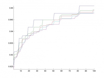
AUC:
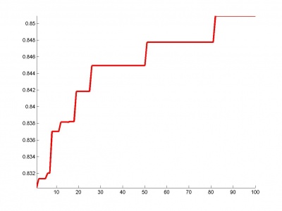
FSS
GA
GMDH
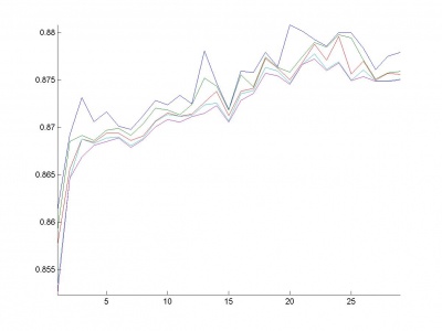
RMSE:
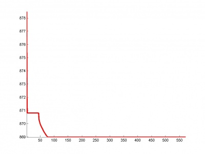
FSS
BSS
FBSS
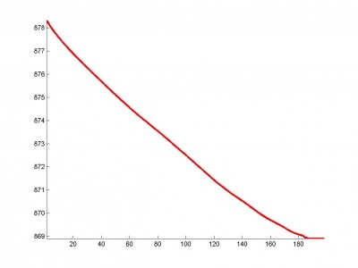
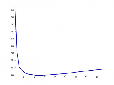
GMDH
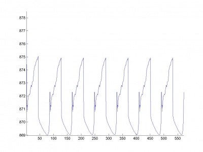
GA
Analysis of Algorithms
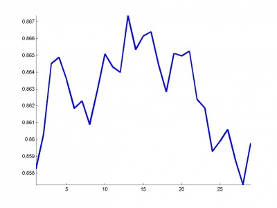
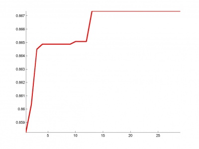
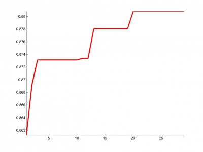
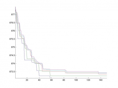
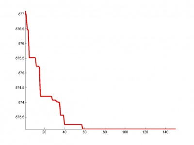
- All algorithms except for the Genetic Search have the parameter NumberOfUnsuccessful-Iterations that is responsible for the number of iterations after the local minimum has been reached. If it is small (~5 iterations), algorithms will miss some solutions that yield better results on a qualifying dataset. For example, let us consider the FSS_AUC task. Based on the right(red) graph we see that minimal possible value of parameter is 35 (the length of the longest segment parallel to the x-axis). If it was less than 35, the FSS would stop without reaching the AUC value 0.8485.
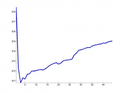
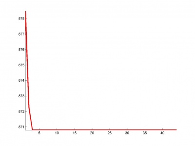
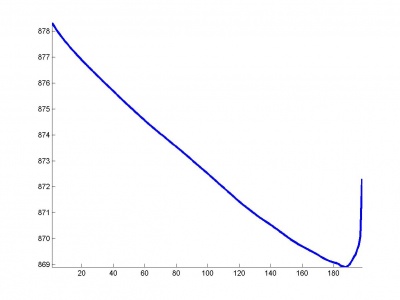
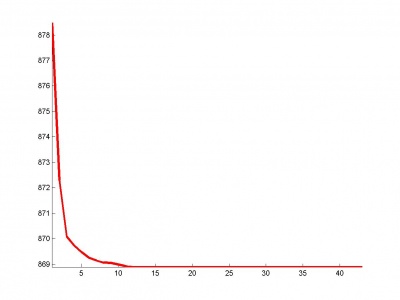
- Let us consider RMSE_FSS, RMSE_BSS and RMSE_GMDH graphs. In FSS and BSS we add probes sequentially and take into account only one best-performed composition. On the other hand, in GMDH we add probes sequentially but now top K models go the next generation. Because of that the functional increases smoother in case of GMDH. It is able to find optimal solution among K models instead of 1 in greedy methods.
Computational Results
Performance measures on a qualifying datasets.
| Algorithm | RMSE | AUC |
|---|---|---|
| Baseline | 878,2381 | 0,88594 |
| FSS | 870,7911 | 0,9304639 |
| BSS | 869,5097 | - |
| FBSS | 869,2673 | - |
| GMDH | 869,4233 | 0,925316 |
| Genetic Search | 874,9305 | 0,9163013 |
Indices of best probes
AUC
FSS: 8,15,33,42,45,49,54,98,143,165,175,179,200
GMDH: 4,24,31,34,38,41,53,61,73,74,78,93,94,105,107,127,130,134,139
GA: 3,4,11,15,22,29,31,37,38,41,46,48,54,58,59,64,69,71,75,79,80,90,92,96,97,98,103, 105,107,108,116,117,118,120,123,125,127,129,131,132,134,136,137,143,144,147,149,154,157, 158,160,165,166,168,169,171,175,177,179,187,190,197
RMSE
FSS: 63,132,137
BSS: 21,26,58,63,117,132,137,183,187,194,196,199
FBSS: 20,21,26,63,132,137,166,183,187,194,199
GMDH: 21,26,58,63,117,132,137,166,183,187,194,199
GA: 1,5,6,7,9,13,14,15,19,20,21,23,24,26,27,28,32,33,35,39,42,43,47,48,50,55, 57,59,63,66,69,70,71,73,74,75,85,87,90,93,94,95,96,99,100,102,103,104,105, 108,110,114,116,117,118,120,121,125,127,131,132,135,136,137,142,143,148,151, 156,157,160,161,162,164,166,167,168,173,174,175,176,179,180,183,187,188,189, 192,193,194,195,196,199,200
References
[1] R. Bell and Y. Koren. Scalable Collaborative Filtering with Jointly Derived Neighborhood Interpolation Weights. IEEE International Conference on Data Mining (ICDM’07), pp. 43–52, 2007.
[2] Breiman L. Bagging predictors // Machine Learning. 1996. Vol. 24, no. 2. Pp. 123–140.
[3] Friedman J., Hastie T., Tibshirani R. Additive logistic regression: a statistical view of boosting: Tech. rep.: Dept. of Statistics, Stanford University Technical Report, 1998.
[4] L. Breiman Heuristics of instability in model selection. Technical report, Statistics Department, University of California at Berkeley, 1994.
[5] R. Caruana, A. Niculescu-Mizil, G. Crew, and A. Ksikes Ensemble selection from libraries of models, In ICML, 2004.
[6] R. Caruana, A. Munson, A. Niculescu-Mizil Getting the Most Out of Ensemble Selection, Technical Report, 2006-2045
System description and report
- Link to the same file in a pdf format
See also
Отчет о выполнении исследовательского проекта (практика, В.В. Стрижов)
| | Данная статья была создана в рамках учебного задания.
См. также методические указания по использованию Ресурса MachineLearning.ru в учебном процессе. |
