Daily electricity price forecasting (report)
Материал из MachineLearning.
(→Set of algorithm variants and modifications) |
|||
| Строка 1: | Строка 1: | ||
| - | + | ==Computing experiment report== | |
| - | == | + | ===Visual analysis=== |
| - | === | + | ====Model data==== |
| - | + | ||
| - | + | ||
| - | + | ||
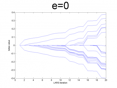
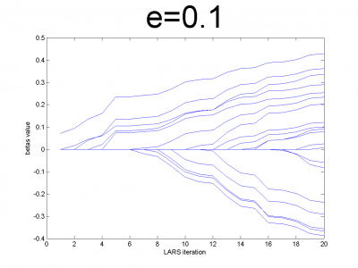
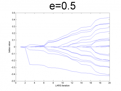
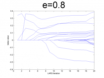
| - | + | At first we have to test our interpretation of LARS to be sure | |
| - | + | about its correct work. LARS has to work better with | |
| - | + | well-conditioned matrix, as many linear algorithms, such as LASSO. | |
| + | For ill-conditioned matrix values of regression coefficients | ||
| + | <tex>\beta</tex> appear to increase and decrease during each step of | ||
| + | algorithm. We generate model data by the below code. | ||
| - | == | + | <code> |
| - | + | n = 100; | |
| - | + | m = 20; | |
| - | + | X = e*ones(n,m)+(1-e)*[diag(ones(m,1));zeros(n-m,m)]; | |
| - | + | beta = (rand(m,1)-0.5); | |
| - | + | Y = X*beta; | |
| - | + | X = X + (rand(n,m) - 0.5)/10; | |
| - | + | ||
| - | + | ||
| - | + | ||
| - | + | ||
| - | + | ||
| - | + | </code> | |
| - | + | ||
| - | + | ||
| - | |||
| - | |||
| - | |||
| - | |||
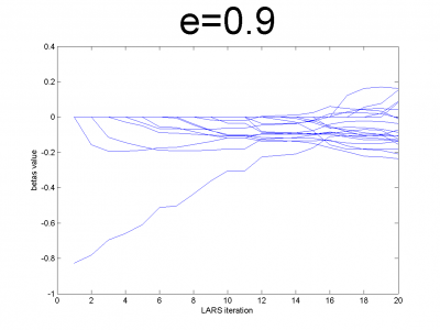
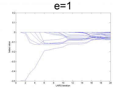
| - | == | + | For different values of <tex>e</tex> we get ill- and well-conditioned |
| - | + | matrices. We use <tex>e=0.1k, k=\overline{1,10}</tex>. If <tex>e</tex> is small | |
| - | + | matrix'll be well-conditioned with close to orthogonal correlation | |
| - | + | vectors, if <tex>e</tex> is close to 1, we get matrix from just ones with | |
| + | little noise. This matrix is ill-conditioned. Directions of | ||
| + | correlation vectors are near to same. | ||
| - | == | + | [[Изображение:EPF_10e=0.png|400px]] |
| + | [[Изображение:EPF_10e=1.png|400px]] | ||
| + | [[Изображение:EPF_10e=5.png|400px]] | ||
| + | [[Изображение:EPF_10e=8.png|400px]] | ||
| + | [[Изображение:EPF_10e=9.png|400px]] | ||
| + | [[Изображение:EPF_10e=10.png|400px]] | ||
| - | |||
| - | |||
| - | |||
| - | |||
| - | |||
| - | + | So, our LARS realization works normal according to this property. | |
| - | + | ||
| - | == | + | ====Data description==== |
| - | + | As real data we use set from our problem. It consists | |
| - | + | from variables matrix <tex>xRegression</tex> and responses vector | |
| - | + | <tex>yRegression</tex>. We will designate them as <tex>X</tex> and <tex>Y</tex>. Size of <tex>X</tex> | |
| - | + | is <tex>n\times m</tex>, where <tex>n</tex> is number of objects (time series from | |
| - | + | days) and <tex>m</tex> is number of variables for each object. Size of <tex>Y</tex> | |
| - | + | is column <tex>n\times 1</tex>. | |
| - | + | ||
| - | + | ||
| - | + | ||
| - | + | ||
| - | + | ||
| - | + | ||
| - | + | ||
| - | + | ||
| - | + | ||
| - | + | ||
| - | + | ||
| - | + | ||
| - | + | ||
| - | + | ||
| - | + | ||
| - | + | ||
| - | + | ||
| - | + | ||
| - | from | + | |
| - | + | ||
| - | + | ||
| - | + | ||
| - | of | + | |
| - | + | ||
| - | + | First column for both <tex>X</tex> and <tex>Y</tex> is time series. For <tex>Y</tex> second | |
| + | column is responses for each object from <tex>X</tex>. They are normalized | ||
| + | by year mean. Number of variables in <tex>X</tex> is 26. They are described | ||
| + | in below table. | ||
| - | + | {| class="wikitable" style="text-align: center;" | |
| + | |- bgcolor="#cccccc" | ||
| + | ! width=30 % |# | ||
| + | ! width=160 % | Description | ||
| - | |||
| - | |||
| - | |||
| - | |||
| - | |||
| - | |||
| - | |||
| - | |||
| - | |||
| - | |||
| - | |||
| - | |||
| - | |||
| - | |||
| - | |||
| - | |||
| - | |||
| - | |||
| - | |||
| - | |||
| - | |||
| - | |||
| - | + | |- | |
| - | + | | '''1''' || time series | |
| - | + | |- | |
| - | + | | '''2-6''' || day of week | |
| - | + | |- | |
| - | + | | '''7-18''' || month | |
| - | week | + | |- |
| - | + | | '''19''' || mean temperature | |
| - | + | |- | |
| - | + | | '''20''' || HDD | |
| - | + | |- | |
| - | + | | '''21''' || CDD | |
| - | + | |- | |
| - | + | | '''22''' || high tepmeratue | |
| - | + | |- | |
| - | + | | '''23''' || low temperature | |
| - | + | |- | |
| - | + | | '''24''' || relative humidity | |
| - | + | |- | |
| - | + | | '''25''' || precipitation | |
| - | + | |- | |
| - | + | | '''26''' || wind speed | |
| - | + | |- | |
| - | + | |} | |
| - | + | ||
| - | + | ||
| - | + | ||
| - | + | ||
| - | + | ||
| - | + | ||
| - | + | ||
| - | + | ||
| - | + | ||
| - | + | ||
| - | + | ||
| - | + | ||
| - | + | ||
| - | + | ||
| - | + | ||
| - | + | ||
| - | + | ||
| - | + | ||
| - | + | ||
| - | + | ||
| - | + | ||
| - | + | ||
| - | + | ||
| - | + | ||
| - | + | ||
| - | + | ||
| - | + | ||
| - | + | ||
| - | + | ||
| - | + | ||
| - | + | ||
| - | + | ||
| - | + | ||
| - | + | ||
| - | + | ||
| - | + | ||
| - | |||
| - | |||
| - | |||
| - | |||
| - | |||
| - | + | ====Experiments with simple LARS==== | |
| + | We do a number of computational experiments with | ||
| + | real data. For each experiment we calculate MAPE value. | ||
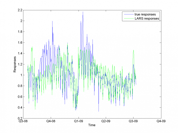
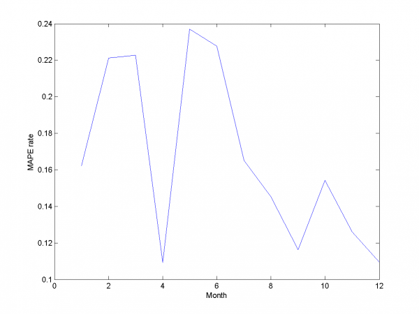
| - | <tex> | + | In first case we use simple LARS algorithm without any additional |
| + | improvements for matrix <tex>X</tex> and column <tex>Y</tex>. | ||
| - | + | <code> | |
| + | model = [1,1,0,0,0,0,0,0,0]; % model parameters | ||
| + | </code> | ||
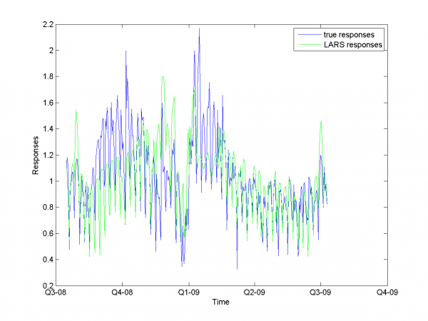
| - | + | [[Изображение:EPF SC LARSresults.png|600px]] | |
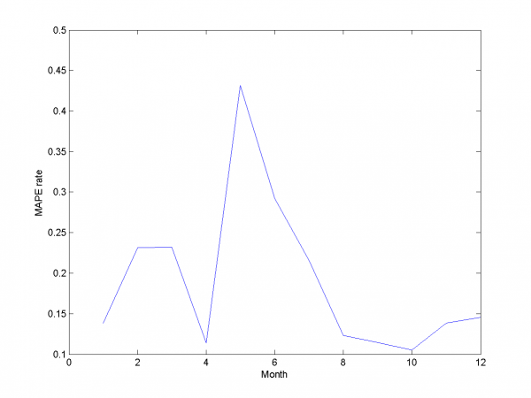
| - | + | [[Изображение:EPF SC MAPEresults.png|600px]] | |
| - | + | ||
| - | + | ||
| - | + | ||
| - | + | ||
| - | + | ||
| - | + | ||
| - | + | Mean MAPE for all months equals 16.64%. | |
| - | + | ||
| - | + | ||
| - | + | ||
| - | + | ||
| - | + | For second experiment we use some additional variables. They are | |
| + | squares and square roots from basic variables | ||
| - | + | <code> | |
| + | model = [1,1,1,0,0,0,0,0,0]; % model parameters | ||
| + | </code> | ||
| - | + | [[Изображение:EPF AV LARSresults.png|600px]] | |
| + | [[Изображение:EPF AV MAPEresults.png|600px]] | ||
| - | + | Mean MAPE for all months equals 17.20%. | |
| - | + | ||
| - | + | In third experiment we use smoothed and indicator variables. | |
| - | + | ||
| - | + | <code> | |
| - | + | model = [1,0,0,1,0,0,0,0,0]; % model parameters | |
| - | + | </code> | |
| - | + | [[Изображение:EPF SS LARSresults.png|600px]] | |
| + | [[Изображение:EPF SS MAPEresults.png|600px]] | ||
| - | + | Mean MAPE equals 17.16%. | |
| + | For the next experiment we choose smoothed and squared smoothed | ||
| + | variables. | ||
| - | = | + | <code> |
| + | model = [1,0,0,1,1,0,0,0,0]; % model parameters | ||
| + | </code> | ||
| - | + | [[Изображение:EPF CS LARSresults.png|600px]] | |
| - | + | [[Изображение:EPF CS MAPEresults.png|600px]] | |
| - | + | ||
| - | + | ||
| - | + | MAPE equals 19.2%. | |
| - | + | In the last experiment of this subsection we choose combination of | |
| - | + | nonsmoothed and smoothed variables. | |
| - | + | <code> | |
| + | model = [1,1,1,1,0,0,0,0,0]; % model parameters | ||
| + | </code> | ||
| - | + | [[Изображение:EPF CSS LARSresults.png|600px]] | |
| - | + | [[Изображение:EPF CSS MAPEresults.png|600px]] | |
| - | + | ||
| - | + | ||
| - | + | We get MAPE 16.89% in this experiment. | |
| - | + | ||
| - | + | ||
| - | + | ||
| - | + | From experiments above we draw a conclusion, that for simple | |
| - | + | linear method LARS MAPE is in bounds of 16-18%. Adding smoothed | |
| - | + | variables can't correct situation. From plots one can see problem | |
| + | of spikes prediction. MAPE for unexpected jumps is bigger, then | ||
| + | MAPE for stationary zones. To increase accuracy of our forecast we | ||
| + | need another methods. | ||
| - | + | ====Removing spikes==== | |
| - | + | To create better forecast we need to remove outliers from learning | |
| - | + | sample. This procedure helps to get better regression | |
| - | + | coefficients. In our case remove spikes procedure depends on our | |
| - | + | basic algorithm model and two parameters. To get optimal value of | |
| - | + | this parameters we use 2 dimensional minimization MAPE procedure. | |
| - | + | First experiment uses initial variables and removing spikes | |
| - | + | procedure. | |
| - | + | ||
| - | + | ||
| - | < | + | <code> |
| - | + | model = [1,1,0,0,0,0,0,0,0]; % model parameters | |
| - | + | </code> | |
| - | + | ||
| - | </ | + | |
| - | + | [[Изображение:EPF P simplePicks.png|600px]] | |
| - | + | ||
| - | <tex> \ | + | Minimum MAPE equals 15.45\%. It is in point |
| + | <tex>\{r_1,r_2\}=\{0.5,0.7\}</tex>. MAPE is smaller, then gained in | ||
| + | previous subsection. | ||
| - | + | In second experiment we use another model. We add modified initial | |
| - | + | variables and smoothed variables. | |
| - | + | ||
| - | + | ||
| - | + | ||
| - | + | ||
| - | + | <code> | |
| - | + | model = [1,1,1,1,0,0,0,0,0]; % model parameters | |
| + | </code> | ||
| - | + | [[Изображение:EPF P compliPicks.png|600px]] | |
| - | + | ||
| - | + | ||
| - | + | ||
| - | = | + | MAPE function has local minimum in point <tex>\{r_1,r_2\}=\{0.8,1.0\}</tex> |
| + | and equals 15.29\%. Let's look to plots for optimal <tex>r_1</tex> and | ||
| + | <tex>r_2</tex>. | ||
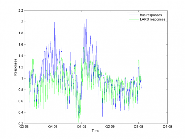
| - | + | [[Изображение:EPF P LARSresults.png|600px]] | |
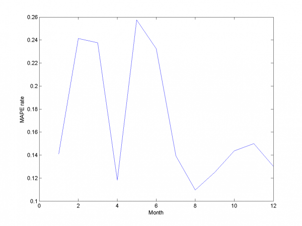
| - | + | [[Изображение:EPF P MAPEresults.png|600px]] | |
| - | + | ||
| - | + | Removing outliers doesn't help us to get better result for months | |
| - | + | with unexpected behavior. To the end of this subsection we note, | |
| + | that this procedure gives us advantage in competition with | ||
| + | previously obtained models and algorithms in previous subsection. | ||
| + | Best MAPE rate for this section experiments is 15.29%. | ||
| - | === | + | ====Autoregression==== |
| + | Add autoregression according to subsection {\bf | ||
| + | 3.4.3} is sound idea for many forecasting algorithms. We use | ||
| + | autoregression in two ways. | ||
| - | + | First way is add to each day from sample responses for days in | |
| - | in matrix | + | past and forecast responses for extended variables matrix. As in |
| - | for | + | previous subsection we use 2-dimensional discrete optimization for |
| - | + | removing spikes parameters. | |
| - | |||
| - | |||
| - | |||
| - | |||
| - | |||
| - | + | \includegraphics[width=0.80\textwidth]{Report/auto/autoPicks.png} | |
| - | + | ||
| - | <tex>{\ | + | We change standard point of view to get more convenient to view |
| + | surface. Minimum MAPE value is in point <tex>\{r_1,r_2\}=\{0.7,0.8\}</tex>. | ||
| + | It equals 13.31\%. | ||
| - | + | <code> | |
| + | model = [1,1,1,1,0,0,0,0.7,0.8]; % model parameters | ||
| + | </code> | ||
| - | + | \includegraphics[width=0.40\textwidth]{Report/auto/LARSresults.png} | |
| - | + | \includegraphics[width=0.40\textwidth]{Report/auto/MAPEresults.png} | |
| - | ==== | + | And for each month: |
| + | \newline | ||
| + | \includegraphics[width=0.90\textwidth]{Report/EachMonth/LARSresults1.png} | ||
| + | \newline | ||
| + | \includegraphics[width=0.90\textwidth]{Report/EachMonth/LARSresults2.png} | ||
| + | \newline | ||
| + | \includegraphics[width=0.90\textwidth]{Report/EachMonth/LARSresults3.png} | ||
| + | \newline | ||
| + | \includegraphics[width=0.90\textwidth]{Report/EachMonth/LARSresults4.png} | ||
| + | \newline | ||
| + | \includegraphics[width=0.90\textwidth]{Report/EachMonth/LARSresults5.png} | ||
| + | \newline | ||
| + | \includegraphics[width=0.90\textwidth]{Report/EachMonth/LARSresults6.png} | ||
| + | \newline | ||
| + | \includegraphics[width=0.90\textwidth]{Report/EachMonth/LARSresults7.png} | ||
| + | \newline | ||
| + | \includegraphics[width=0.90\textwidth]{Report/EachMonth/LARSresults8.png} | ||
| + | \newline | ||
| + | \includegraphics[width=0.90\textwidth]{Report/EachMonth/LARSresults9.png} | ||
| + | \newline | ||
| + | \includegraphics[width=0.90\textwidth]{Report/EachMonth/LARSresults10.png} | ||
| + | \newline | ||
| + | \includegraphics[width=0.90\textwidth]{Report/EachMonth/LARSresults11.png} | ||
| + | \newline | ||
| + | \includegraphics[width=0.90\textwidth]{Report/EachMonth/LARSresults12.png} | ||
| - | |||
| - | |||
| - | |||
| - | |||
| - | + | For this experiment we have best results from our set of different | |
| + | models algorithm. But to complete article it's necessary to | ||
| + | analyze work for other algorithm and models we have use during | ||
| + | work. | ||
| - | + | ====Set of models for each day of week==== | |
| - | + | In data set with periodics can be suitable create it's | |
| - | + | own model for each element from periodic. For example, we can | |
| - | + | create different regression models for different dais of week. | |
| - | + | Work of this heuristic in our case seems interesting. | |
| - | + | ||
| - | for each | + | |
| - | + | ||
| - | + | ||
| - | + | ||
| - | + | ||
| - | + | ||
| - | + | ||
| - | + | ||
| - | + | In experiments we split in two parts: for control and for test. We | |
| + | forecast 4 day of week forward for each day. So, we create for | ||
| + | each crossvalidation forecast for 28 days. | ||
| - | In | + | In first case we create model from standard variables. We test our |
| - | from variables | + | sample with different size of test sample (by what we choose best |
| - | + | <tex>\beta</tex>). Motivation of this step is small number of elements in | |
| + | control sample. It equals 4. But for different sizes of test set | ||
| + | there is no decreasing of MAPE effect. | ||
| - | < | + | <code> |
| - | + | model = [1,1,1,1,0,0,0,0,0,s]; % model parameters | |
| - | </ | + | </code> |
| - | + | <tex>S</tex> is multitude to create size of test sample. Size of test set | |
| - | + | equals <tex>5\cdot s</tex>. | |
| - | + | ||
| - | + | ||
| - | + | ||
| - | + | ||
| - | <tex> | + | |
| - | + | ||
| - | + | \begin{tabular}{|c|c|c|c|c|c|} | |
| - | + | ||
| - | + | ||
| - | + | ||
| - | + | ||
| - | + | ||
| - | + | ||
| - | + | ||
| - | + | ||
| - | + | ||
| - | + | ||
| - | + | ||
| - | + | ||
| - | + | \hline Control set size&4&8&12&16&20 \\ | |
| - | + | \hline MAPE rate&0.1740&0.1860&0.1790&0.1897&0.1846 \\ | |
| - | + | \hline Control set size&24&28&32&36&40 \\ | |
| + | \hline MAPE rate&0.1826&0.1882&0.1831& 0.1846&0.1952 \\ | ||
| + | \hline | ||
| + | \end{tabular} | ||
| - | + | From this table one can see, that results for this experiment | |
| + | aren't better, then results for model without choosing individual | ||
| + | model for each day of week. | ||
| - | + | Let's add autoregression matrix to this model according to way we | |
| - | + | describe in {\bf 3.4.3}. We get <tex>\{ r_1,r_2 \}=\{ 0.3,0.3\}</tex> from | |
| - | + | two-dimensional optimization by this parameters. | |
| - | + | ||
| - | + | ||
| - | + | ||
| - | + | \includegraphics[width=0.80\textwidth]{Report/autoDOW/autoPicks.png} | |
| - | + | We got results below. MAPE equals 14.79\%. | |
| - | < | + | <code> |
| + | model = [1,1,1,0,0,0,6,0.3,0.3,1]; % model parameters | ||
| + | </code> | ||
| - | + | \includegraphics[width=0.40\textwidth]{Report/autoDOW/LARSresults.png} | |
| - | + | \includegraphics[width=0.40\textwidth]{Report/autoDOW/MAPEresults.png} | |
| - | + | ||
| - | + | ||
| + | To the end of this section we say, that for our data set this way | ||
| + | can't give us as precise results as method from previous section. | ||
| - | ==== | + | ==== Local algorithm Fedorovoy==== |
| + | For algorithm Fedorovoy we don't use any additional | ||
| + | hypotheses except described in works \cite{[11]},\cite{[12]}. | ||
| + | Results for this algorithm are worse, that result for different | ||
| + | LARS variations. Main complications in our data for this algorithm | ||
| + | are big noises and spikes in learning and test data set and weak | ||
| + | dependence future data from past. Motivation to use this algorithm | ||
| + | is periodics in our data. | ||
| - | + | To get parameters for this algorithm we have used iteration | |
| - | is | + | method. At first iteration we got local minimum in point <tex>\{ k,\om |
| + | \}=\{49, 0.9\}</tex>, where <tex>k</tex> is number of nearest neighbours for our | ||
| + | algorithm and <tex>\om</tex> defines way to calculate distance between | ||
| + | different segments of our sample. | ||
| - | + | \includegraphics[width=0.40\textwidth]{Report/Local/kNNresults.png} | |
| - | + | \includegraphics[width=0.40\textwidth]{Report/Local/MAPEresults.png} | |
| - | + | MAPE equals 20.43\%. | |
| - | + | ||
| - | + | ||
| - | === | + | ===Criterion analysis=== |
| - | + | We use MAPE quality functional. In our case target function to | |
| - | + | minimize is deviation of initial responses to ones from algorithm, | |
| - | + | so this functional looks suitable. For many variations and 2 | |
| - | + | algorithms we got set of different results. Let's briefly describe | |
| + | them in the table. | ||
| - | + | \begin{tabular}{|c|c|c|c|c|c|} | |
| - | + | \hline Algorithm&LARS&RS LARS& RS and autoLARS& DOW LARS& LAF \\ | |
| - | + | \hline MAPE&16.64\%&15.29\%&{\bf 13.31\%}&14.79\%&20.43\% \\ | |
| + | \hline | ||
| + | \end{tabular} | ||
| - | + | {\it LARS} is simple LARS realization with best set of variables. | |
| - | + | {\it AutoLARS} is LARS with removing spikes procedure. {\it RS and | |
| - | + | autoLARS} is LARS with removing spikes and adding autoregression | |
| + | variables. {\it DOW LARS} is LARS with creation specified model | ||
| + | for each periodic (in our case -- week periodic). For this | ||
| + | algorithm we also add autoregression variables and remove spikes | ||
| + | procedure.{\it LAF} is local algorithm Fedorovoy realization. For | ||
| + | our variants of this algorithms set we get best result with {\it | ||
| + | RS and autoLARS}. | ||
| - | + | Main complication for most of algorithm was spikes and outliers in | |
| + | data set. Another complication for LARS-based algorithm was weak | ||
| + | correlation between initial variables and responses. To this | ||
| + | problem we add also high rate of noise. The reason of it can be | ||
| + | unobservable in our data events. Some from our algoithms take into | ||
| + | account this complications. They gave us better results, then | ||
| + | simple algorithms. But we get only 4-5\% of MAPE rate by applying | ||
| + | our best algorithm in complication with simple LARS. | ||
| - | === | + | ===Dependency from parameters analysis=== |
| - | + | In different sections of our work we use a number of optimization | |
| + | procedures. Frow plots and 3d plots one can see, that all | ||
| + | optimizations are stabile and give us close to optimal parameters. | ||
| + | In most algorithms we use simple discrete one- or two-dimensional | ||
| + | optimization. For local algorithm Fedorovoy we use iterations | ||
| + | method, but he gives us local optimum result at first step. May | ||
| + | be, it's suitable to apply randomization search in this case. | ||
| - | == | + | ==Results report== |
| - | + | For our best algorithm we decrease MAPE rate by 5\% from initial | |
| + | algorithm (We get 13.31\% MAPE rate vs 17\% in start). To solve | ||
| + | this problem we applied big set of heuristics and modifications to | ||
| + | LARS. We also created realization of local algorithm | ||
| + | k-nearest-neighbours to compare results. | ||
== Список литературы == | == Список литературы == | ||
Версия 08:17, 14 февраля 2010
Computing experiment report
Visual analysis
Model data
At first we have to test our interpretation of LARS to be sure
about its correct work. LARS has to work better with
well-conditioned matrix, as many linear algorithms, such as LASSO.
For ill-conditioned matrix values of regression coefficients
appear to increase and decrease during each step of
algorithm. We generate model data by the below code.
n = 100;
m = 20;
X = e*ones(n,m)+(1-e)*[diag(ones(m,1));zeros(n-m,m)];
beta = (rand(m,1)-0.5);
Y = X*beta;
X = X + (rand(n,m) - 0.5)/10;
For different values of we get ill- and well-conditioned
matrices. We use
. If
is small
matrix'll be well-conditioned with close to orthogonal correlation
vectors, if
is close to 1, we get matrix from just ones with
little noise. This matrix is ill-conditioned. Directions of
correlation vectors are near to same.
So, our LARS realization works normal according to this property.
Data description
As real data we use set from our problem. It consists
from variables matrix and responses vector
. We will designate them as
and
. Size of
is
, where
is number of objects (time series from
days) and
is number of variables for each object. Size of
is column
.
First column for both and
is time series. For
second
column is responses for each object from
. They are normalized
by year mean. Number of variables in
is 26. They are described
in below table.
| # | Description
|
|---|---|
| 1 | time series |
| 2-6 | day of week |
| 7-18 | month |
| 19 | mean temperature |
| 20 | HDD |
| 21 | CDD |
| 22 | high tepmeratue |
| 23 | low temperature |
| 24 | relative humidity |
| 25 | precipitation |
| 26 | wind speed |
Experiments with simple LARS
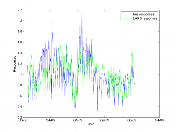
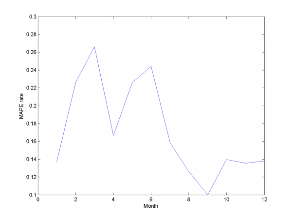
We do a number of computational experiments with real data. For each experiment we calculate MAPE value.
In first case we use simple LARS algorithm without any additional
improvements for matrix and column
.
model = [1,1,0,0,0,0,0,0,0]; % model parameters
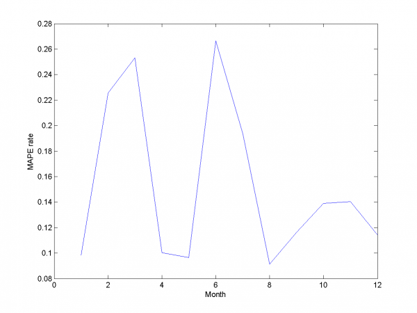
Mean MAPE for all months equals 16.64%.
For second experiment we use some additional variables. They are squares and square roots from basic variables
model = [1,1,1,0,0,0,0,0,0]; % model parameters
Mean MAPE for all months equals 17.20%.
In third experiment we use smoothed and indicator variables.
model = [1,0,0,1,0,0,0,0,0]; % model parameters
Mean MAPE equals 17.16%.
For the next experiment we choose smoothed and squared smoothed variables.
model = [1,0,0,1,1,0,0,0,0]; % model parameters
MAPE equals 19.2%.
In the last experiment of this subsection we choose combination of nonsmoothed and smoothed variables.
model = [1,1,1,1,0,0,0,0,0]; % model parameters
We get MAPE 16.89% in this experiment.
From experiments above we draw a conclusion, that for simple linear method LARS MAPE is in bounds of 16-18%. Adding smoothed variables can't correct situation. From plots one can see problem of spikes prediction. MAPE for unexpected jumps is bigger, then MAPE for stationary zones. To increase accuracy of our forecast we need another methods.
Removing spikes
To create better forecast we need to remove outliers from learning sample. This procedure helps to get better regression coefficients. In our case remove spikes procedure depends on our basic algorithm model and two parameters. To get optimal value of this parameters we use 2 dimensional minimization MAPE procedure.
First experiment uses initial variables and removing spikes procedure.
model = [1,1,0,0,0,0,0,0,0]; % model parameters
Изображение:EPF P simplePicks.png
Minimum MAPE equals 15.45\%. It is in point
. MAPE is smaller, then gained in
previous subsection.
In second experiment we use another model. We add modified initial variables and smoothed variables.
model = [1,1,1,1,0,0,0,0,0]; % model parameters
Изображение:EPF P compliPicks.png
MAPE function has local minimum in point
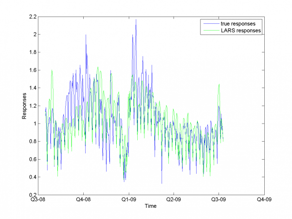
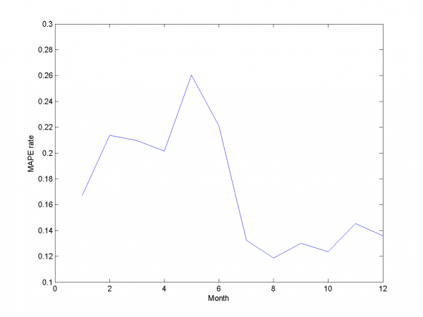
and equals 15.29\%. Let's look to plots for optimal
and
.
Removing outliers doesn't help us to get better result for months with unexpected behavior. To the end of this subsection we note, that this procedure gives us advantage in competition with previously obtained models and algorithms in previous subsection. Best MAPE rate for this section experiments is 15.29%.
Autoregression
Add autoregression according to subsection {\bf 3.4.3} is sound idea for many forecasting algorithms. We use autoregression in two ways.
First way is add to each day from sample responses for days in past and forecast responses for extended variables matrix. As in previous subsection we use 2-dimensional discrete optimization for removing spikes parameters.
\includegraphics[width=0.80\textwidth]{Report/auto/autoPicks.png}
We change standard point of view to get more convenient to view
surface. Minimum MAPE value is in point .
It equals 13.31\%.
model = [1,1,1,1,0,0,0,0.7,0.8]; % model parameters
\includegraphics[width=0.40\textwidth]{Report/auto/LARSresults.png} \includegraphics[width=0.40\textwidth]{Report/auto/MAPEresults.png}
And for each month: \newline \includegraphics[width=0.90\textwidth]{Report/EachMonth/LARSresults1.png} \newline \includegraphics[width=0.90\textwidth]{Report/EachMonth/LARSresults2.png} \newline \includegraphics[width=0.90\textwidth]{Report/EachMonth/LARSresults3.png} \newline \includegraphics[width=0.90\textwidth]{Report/EachMonth/LARSresults4.png} \newline \includegraphics[width=0.90\textwidth]{Report/EachMonth/LARSresults5.png} \newline \includegraphics[width=0.90\textwidth]{Report/EachMonth/LARSresults6.png} \newline \includegraphics[width=0.90\textwidth]{Report/EachMonth/LARSresults7.png} \newline \includegraphics[width=0.90\textwidth]{Report/EachMonth/LARSresults8.png} \newline \includegraphics[width=0.90\textwidth]{Report/EachMonth/LARSresults9.png} \newline \includegraphics[width=0.90\textwidth]{Report/EachMonth/LARSresults10.png} \newline \includegraphics[width=0.90\textwidth]{Report/EachMonth/LARSresults11.png} \newline \includegraphics[width=0.90\textwidth]{Report/EachMonth/LARSresults12.png}
For this experiment we have best results from our set of different
models algorithm. But to complete article it's necessary to
analyze work for other algorithm and models we have use during
work.
Set of models for each day of week
In data set with periodics can be suitable create it's own model for each element from periodic. For example, we can create different regression models for different dais of week. Work of this heuristic in our case seems interesting.
In experiments we split in two parts: for control and for test. We forecast 4 day of week forward for each day. So, we create for each crossvalidation forecast for 28 days.
In first case we create model from standard variables. We test our
sample with different size of test sample (by what we choose best
). Motivation of this step is small number of elements in
control sample. It equals 4. But for different sizes of test set
there is no decreasing of MAPE effect.
model = [1,1,1,1,0,0,0,0,0,s]; % model parameters
is multitude to create size of test sample. Size of test set
equals
.
\begin{tabular}{|c|c|c|c|c|c|}
\hline Control set size&4&8&12&16&20 \\ \hline MAPE rate&0.1740&0.1860&0.1790&0.1897&0.1846 \\ \hline Control set size&24&28&32&36&40 \\ \hline MAPE rate&0.1826&0.1882&0.1831& 0.1846&0.1952 \\ \hline \end{tabular}
From this table one can see, that results for this experiment aren't better, then results for model without choosing individual model for each day of week.
Let's add autoregression matrix to this model according to way we
describe in {\bf 3.4.3}. We get from
two-dimensional optimization by this parameters.
\includegraphics[width=0.80\textwidth]{Report/autoDOW/autoPicks.png}
We got results below. MAPE equals 14.79\%.
model = [1,1,1,0,0,0,6,0.3,0.3,1]; % model parameters
\includegraphics[width=0.40\textwidth]{Report/autoDOW/LARSresults.png} \includegraphics[width=0.40\textwidth]{Report/autoDOW/MAPEresults.png}
To the end of this section we say, that for our data set this way can't give us as precise results as method from previous section.
Local algorithm Fedorovoy
For algorithm Fedorovoy we don't use any additional hypotheses except described in works \cite{[11]},\cite{[12]}. Results for this algorithm are worse, that result for different LARS variations. Main complications in our data for this algorithm are big noises and spikes in learning and test data set and weak dependence future data from past. Motivation to use this algorithm is periodics in our data.
To get parameters for this algorithm we have used iteration
method. At first iteration we got local minimum in point , where
is number of nearest neighbours for our
algorithm and
defines way to calculate distance between
different segments of our sample.
\includegraphics[width=0.40\textwidth]{Report/Local/kNNresults.png} \includegraphics[width=0.40\textwidth]{Report/Local/MAPEresults.png}
MAPE equals 20.43\%.
Criterion analysis
We use MAPE quality functional. In our case target function to minimize is deviation of initial responses to ones from algorithm, so this functional looks suitable. For many variations and 2 algorithms we got set of different results. Let's briefly describe them in the table.
\begin{tabular}{|c|c|c|c|c|c|}
\hline Algorithm&LARS&RS LARS& RS and autoLARS& DOW LARS& LAF  \\
\hline MAPE&16.64\%&15.29\%&{\bf 13.31\%}&14.79\%&20.43\% \\
\hline
\end{tabular}
{\it LARS} is simple LARS realization with best set of variables. {\it AutoLARS} is LARS with removing spikes procedure. {\it RS and autoLARS} is LARS with removing spikes and adding autoregression variables. {\it DOW LARS} is LARS with creation specified model for each periodic (in our case -- week periodic). For this algorithm we also add autoregression variables and remove spikes procedure.{\it LAF} is local algorithm Fedorovoy realization. For our variants of this algorithms set we get best result with {\it RS and autoLARS}.
Main complication for most of algorithm was spikes and outliers in data set. Another complication for LARS-based algorithm was weak correlation between initial variables and responses. To this problem we add also high rate of noise. The reason of it can be unobservable in our data events. Some from our algoithms take into account this complications. They gave us better results, then simple algorithms. But we get only 4-5\% of MAPE rate by applying our best algorithm in complication with simple LARS.
Dependency from parameters analysis
In different sections of our work we use a number of optimization procedures. Frow plots and 3d plots one can see, that all optimizations are stabile and give us close to optimal parameters. In most algorithms we use simple discrete one- or two-dimensional optimization. For local algorithm Fedorovoy we use iterations method, but he gives us local optimum result at first step. May be, it's suitable to apply randomization search in this case.
Results report
For our best algorithm we decrease MAPE rate by 5\% from initial algorithm (We get 13.31\% MAPE rate vs 17\% in start). To solve this problem we applied big set of heuristics and modifications to LARS. We also created realization of local algorithm k-nearest-neighbours to compare results.
Список литературы
| | Данная статья является непроверенным учебным заданием.
До указанного срока статья не должна редактироваться другими участниками проекта MachineLearning.ru. По его окончании любой участник вправе исправить данную статью по своему усмотрению и удалить данное предупреждение, выводимое с помощью шаблона {{Задание}}. См. также методические указания по использованию Ресурса MachineLearning.ru в учебном процессе. |
